Transformations in R

For this example we will use data on the number of electronic academic journals over a seven-year period. Note the shortcut for entering consecutive years. The journal counts were cut and pasted from another statistical software package after invoking the scan function (and hitting Return). There are so few you could just type them in.

> year = c(1991:1997)
> year
[1] 1991 1992 1993 1994 1995 1996 1997
> Journals <- scan()
1: 27
2: 36
3: 45
4: 181
5: 306
6: 1093
7: 2459
8: 
Read 7 items

> plot(year,Journals)

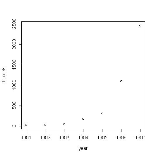
Not surprisingly, the number of electronic journals really took off during this period. Sometimes "exponential growth" is used to describe any kind of rapid growth, but technically it refers to a specific mathematical pattern. If we have true exponential growth, then plotting the logarithms of the growing variable versus time should give a straight line. First take the logarithms, then make the plot.

> logJ=log(Journals)
 > plot(year,logJ)

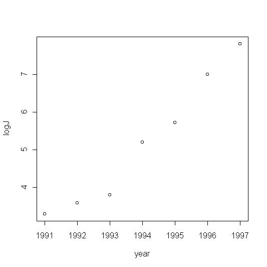
The original graph shows strong curvature. The logarithms of the journal counts plot as much more linear versus year. We might say that the growth is approximately exponential, especially after the first year.

It might be interesting to see the effect of the transformation on the journal counts considered by themselves.

> hist(Journals)
> hist(logJ)

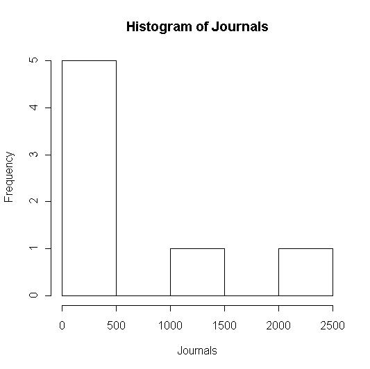
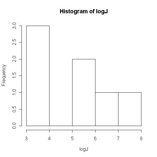
Here the transformation makes the data much less skewed.

Logarithms are a common transformation but certainly not the only one. We can do simple arithmetic transformations at the command line. For example, it is not clear whether fuel efficiency should be measured in miles per gallon or gallons per mile. If we have data in one form in a variable MPG, a reciprocal transformation takes us to the other.

> GPM=1/MPG