This example uses data on the heights (in mm) of married couples. The data were supplied in two plain ASCII text files, husbands.txt and wives.txt. Open one of the files in an ASCII text editor such as Notepad, SimpleText or Emacs. Browse through it to make sure everything is OK. In the original data source there was a blank line after observation 50 and another blank line further down. R would interpret the first of these as the end of the dataset and only receive the first 50 observations (out of 199). So, we fixed this in the editor (so you won't have to do that) and then pasted the gap-free columns (one by one) into R. Use the scan function as shown below. Type the command, then Enter, and at the 1: prompt, paste in the data for that variable. Then repeat for the other variable (in the other file). In the printout below, only the first five values for each variable are shown. The length command is used to determine how many values were read.
> wHts <- scan()
1: 1590
2: 1560
3: 1620
4: 1540
5: 1420
> hHts <- scan()
1: 1809
2: 1841
3: 1659
4: 1779
5: 1616
> length(wHts)
[1] 199
> cor(hHts,wHts)
[1] 0.3644337
> plot(hHts,wHts)
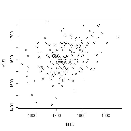
The scatterplot shows a moderate upwards trend with lots of variability, consistent with a correlation of 0.36.
© 2006 Robert W. Hayden