When categorical data appear in textbooks, it is usually already summarized in tables or graphs. Hence, you usually do not need technology to do homework problems with categorical data. However, this leaves one underprepared for dealing with real data, so this page is for those who need to do that. We will use an example dataset small enough so you can do the calculations by hand and compare your results to the computer. Imagine a survey question with answer choices Agree, Disagree or Undecided. Suppose 25 people give these responses:
A,A,D,U,D,D,A,U,A,D,A,D,D,A,U,A,U,D,D,A,A,A,U,D,A.
Most software will not report the mode. That's because the mode is rarely useful for measurements. To find it when you do need it, you have to treat the data as categorical. For categorical data, the modal category is the one with the most observations (if there is such a category). You can see by counting that there are more A's on the list above than D's or U's, so A is the modal category. This is the shortest summary for categorical data, analogous to just giving the mean or median for measurements. When we find the modal category for a group of measurements, it is called the mode. It is useful only when the measurements resemble categorical data in having values that are repeated over and over. An example might be number of children in a family. Here you might see 0, 1, 2... over and over. For more typical measurements, such as these
1.66597, 1.91566, 2.53406, 2.88043, 2.93449, 3.08816, 1.73520, 3.21908, 3.77892, 3.98208
the mode is not useful because there is none. No value is repeated.
If you need the mode, make a frequency table for the data and find the category with the most observations.
Run R and R-Commander. From the R-Commander menu, select Data > New Dataset. Give the new file a name, click OK, and a spreadsheet-like window will open and you can type in your data. Close this window when you are done. From the R-Commander window, select Statistics > Summaries > Frequency distributions.. Though you only have one variable, you still have to click on it to select it. Click on the OK button and tables will appear in the bottom half of the R-Commander window.
> .Table  # counts

 A  D  U
11  9  5

> 100*.Table/sum(.Table)  # percentages

 A  D  U
44 36 20
The modal category (with 44% of the responses) is "Agree".
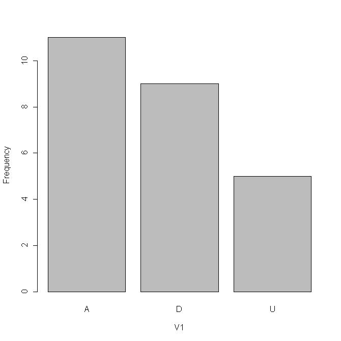
To get a bar chart, select Graphs > Bar graph. Though you only have one variable, you still have to click on it to select it. Click on the OK button and a bar chart will pop up.
To get a pie chart, select Graphs > Pie chart. Though you only have one variable, you still have to click on it to select it. Click on the OK button and a pie chart will pop up.
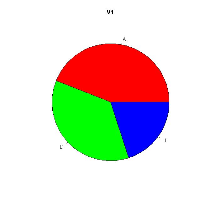
Notice that it is obvious from the bar chart that A is the modal category. It takes sharp eyes to see this in the pie chart. The summaries above are in order of decreasing statistical quality. A table gives the most and most precise information in the least amount of space; a pie chart gives the least.